Machine learning has established connections with a wide range of subjects owing to its versatility and potency. It is now intertwined with all disciplines, finding applicability in areas like automation and optimization, predictive analytics, and personalization and recommendation systems. So let us dive into ML, specifically in this post, SML. 

 In this post, we will be talking about, (CLICK TO JUMP)

• Supervised Machine Learning
• Supervised Learning Algorithms
• Logistic Regression
• Naive Bayes
• Decision Tree

Supervised Machine Learning

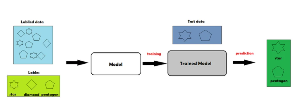
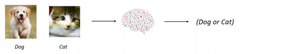
In supervised learning, we have a smart model that learns from examples. Imagine you have a bunch of pictures and you want the model to learn how to recognize different objects in those pictures. To teach it, you also provide labels or tags that tell the model what each object is in the pictures.

The supervised machine learning mechanism

So, the model looks at the pictures and their labels together, and it tries to figure out the patterns and connections between the pictures and their labels. It learns from this labelled data, just like a student learns from a teacher

Once the model has learned from the labelled data, it can use its knowledge to predict the labels for new, unseen pictures. It’s like the model becomes a teacher itself, making predictions based on what it learned before. In a nutshell, supervised learning is like having a teacher show you examples with labels, and then you use that knowledge to make predictions on new things. The labelled data acts as the teacher guiding the model’s learning process. The labelled output data that we have previously input serves as a supervisor for the data we want to predict

Supervised learning can be fundamentally divided into two types.

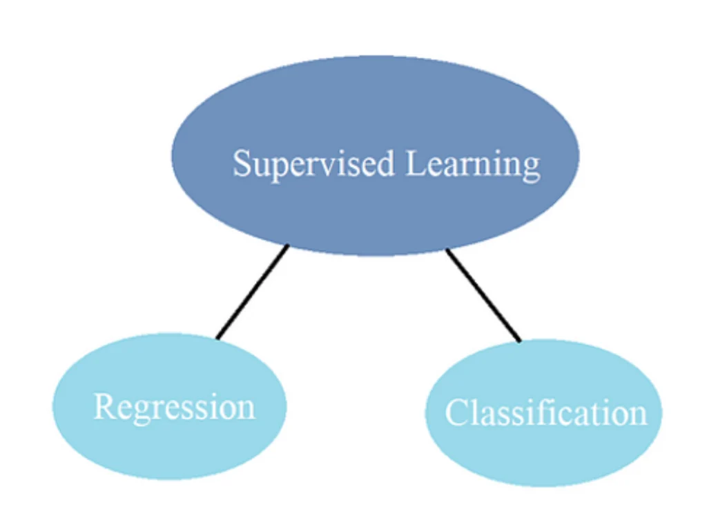
1. Regression
2. Classification

In the world of machine learning, we encounter different types of data that we want to predict. This data can be divided into two main categories: quantitative and qualitative.

Quantitative data is all about numbers and continuous information. It includes things like salaries, prices, weather forecasts, and market trends. When we want to predict these kinds of numeric values, we use a technique called regression. Regression helps us make educated guesses about what the values might be based on patterns and trends in the data.

On the other hand, qualitative data involves classifying things into different categories or discrete values. For example, we might want to predict someone’s gender or whether a statement is true or false. In this case, we use a technique called classification. Classification helps us assign labels or categories to the data based on patterns we observe.

In conclusion, classification is used to predict discrete categories or values and regression is used to predict continuous numeric values. We can evaluate many sorts of data and generate reliable forecasts with the aid of these tools.

Regression

Machine learning uses a variety of regression techniques extensively. Among them are,

1. Linear Regression
2.  Ridge Regression
3. Neural Network Regression
4. Lasso Regression
5. Decision Tree Regression
6. Random Forest
7. KNN Model
8. Support Vector Machines (SVM)
9. Gaussian Regression
10. Polynomial Regression

Classification

Let’s explore some of the widely used and popular classification algorithms in machine learning. These algorithms are powerful tools that help us categorize and classify data based on patterns and features. Here are a few examples:

1. Logistic Regression
2. Naive Bayes
3. K-Nearest Neighbors
4. Decision Tree
5. Support Vector Machines

These are only a few instances of well-known classification algorithms, each of which has advantages and disadvantages. It’s critical to select the appropriate algorithm based on the specifics of the dataset and the nature of the problem. These algorithms allow us to use our data to generate precise forecasts and get insightful knowledge.

By illustrating the training of several of these models, we’ll get into the practical aspect of machine learning in this post. We’ll specifically look at decision trees, random forests, naive bayes, and logistic regression. These simple yet efficient algorithms can aid in the accurate classification and categorization of data.

Logistic Regression

Logistic regression is a mathematical calculation that helps us make these binary predictions. It analyzes independent variables or factors to determine the likelihood of the binary outcome and this logistic function is represented by the following formulas:

Logit(pi) = 1/(1+ exp(-pi))

In this logistic regression equation, logit(pi) is the dependent or response variable and x is the independent variable.

These independent variables can be either categorical (such as types of products, colours, etc.) or numeric (such as age, temperature, etc.). 

However, the dependent variable, the one we want to predict, is always categorical and falls into one of the two binary categories. By considering the relationships and patterns between the independent variables and the binary outcome, logistic regression allows us to estimate the probability of an event occurring or not occurring. This estimation is based on a logistic function, which maps the input data to a probability value between 0 and 1.

Let us start training a model with an example data set, creditcard.csv. In this demonstration, we will train a model to detect fraud credit card detection.

1. Understanding the data

Create a new notebook in Google Colab

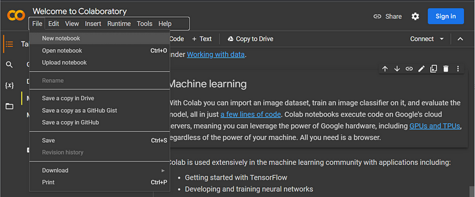
Getting a New notebook in Google Colab

Add new code/text lines whenever wanted

Let’s start to play with our data set. First, we get the basic necessary libraries.

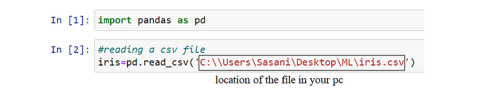
Now, we need to add the .csv file to Colab. And copy the file’s path

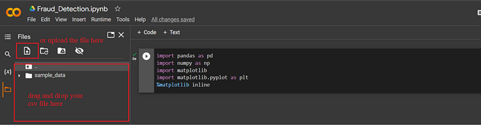
Add the files to Colab

file path

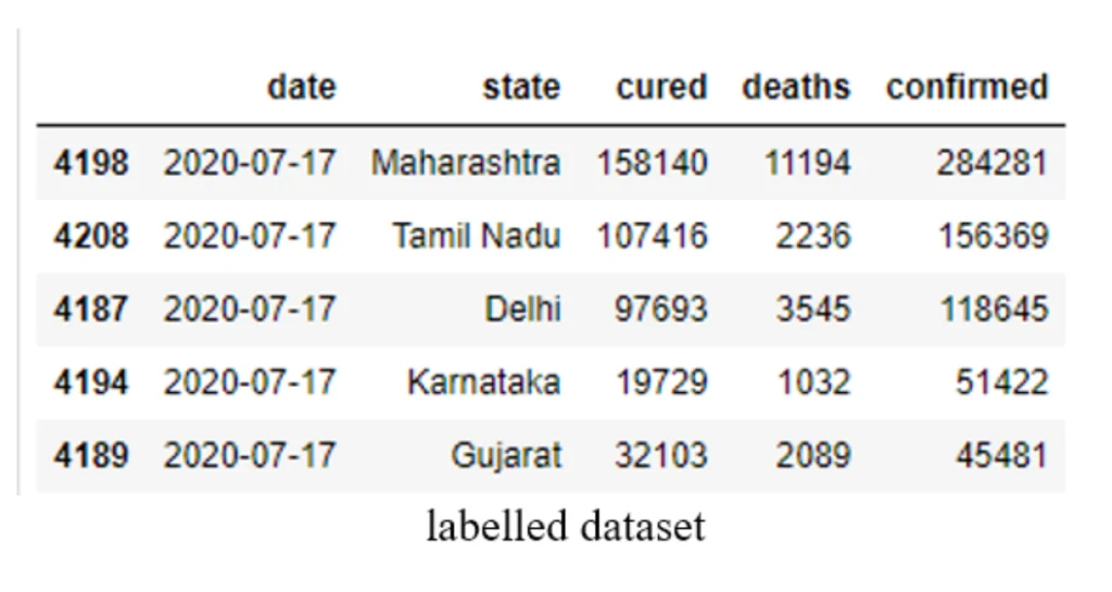
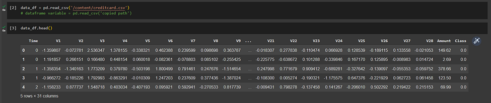
Then we extract the data in the .csv file to a data frame named, ‘data_df’ 
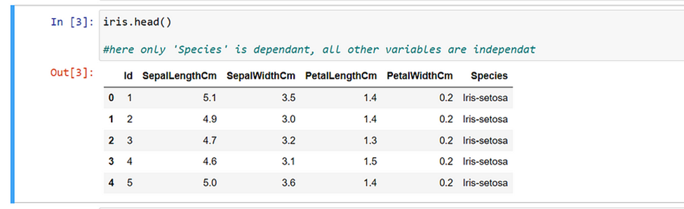
(pandas.read_csv)and print the firstmost elements to get an idea about the dataset (pandas.DataFrame.head).

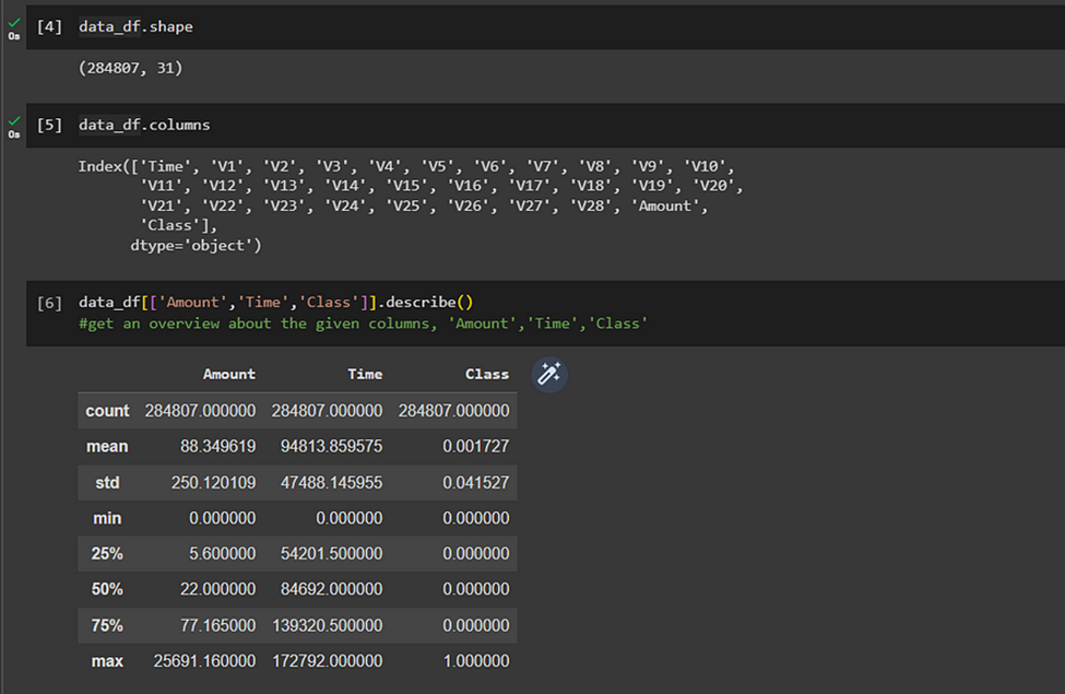
We can get a clear idea about the number of columns and the independent/dependent variables in the data frame. Here in this case our ‘Class’ column is the dependent variable and all the other columns are independent variables. To get a better understanding of the data, we can use the following commands.
pandas.DataFrame.shape, pandas.DataFrame.columns, pandas.DataFrame.describe

2. Detect any possible missing values

When we are using a dataset to train a model, we must provide a proper complete dataset. If our dataset contains NULL values the model would not be accurate. So, we must confirm that our dataset does not contain any NULL values. 

If there are null values present: return TRUE
If there are no null values present: returns False

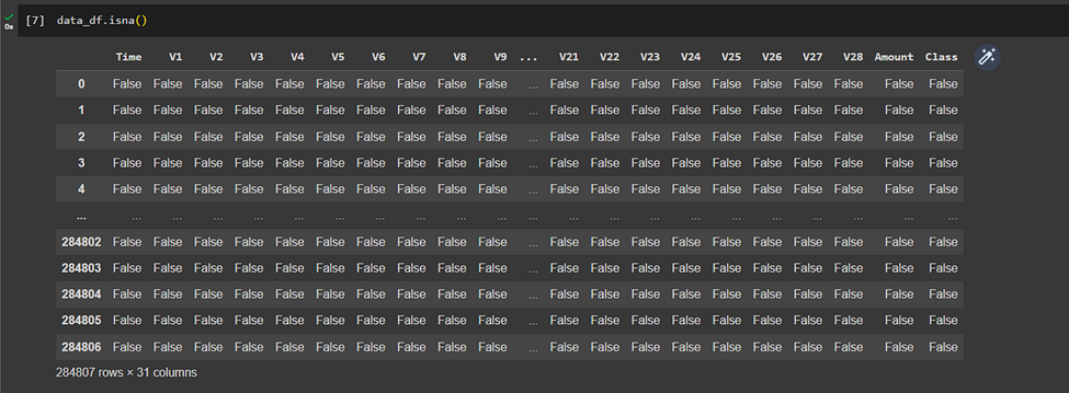
(pandas.DataFrame.isna: returns all cells)

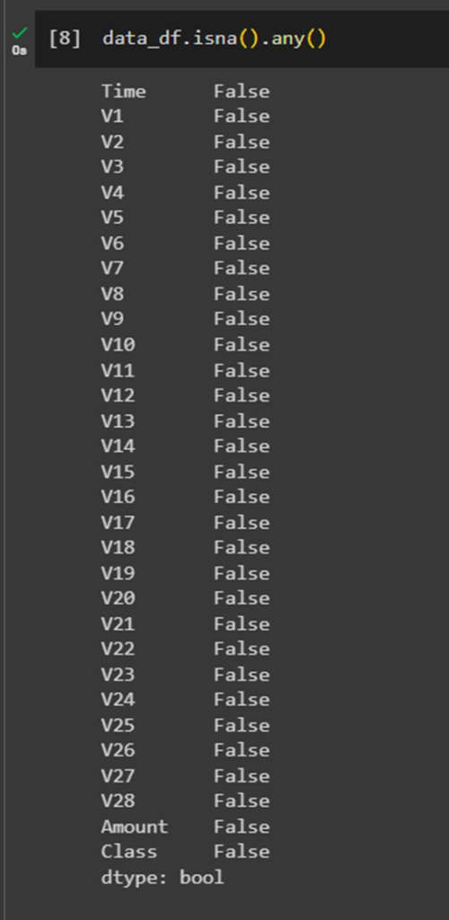
returns the columns, considering all cells in that column

Luckily, in this dataset, we do not have any null values. But, if any case you do have null values, we can replace those null values with “np.nan” and then drop the rows and columns with the value NaN.\

data_df.replace('', np.nan) #replace all null values by NaN

data_df = data_df.dropna(axis=0) #drop row
data_df = data_df.dropna(axis=1) #drop column

null_columns=pd.DataFrame({'Columns':data_df.isna().sum().index,'No. Null Values':data_df.isna().sum().values,'Percentage':data_df.isna().sum().values/data_df.shape[0]})
null_columns #check each column to see if they contain any null cells
data_df.isna().any()

3. Model training data preparation

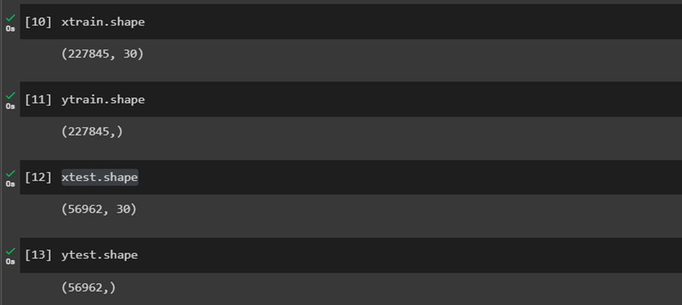
Now we have a complete dataset. We divide this data set into two parts training data and test data.
80% of the data set -> training data
20% of the data set -> test data (the percentage can be customized accordingly)

Using train_test_split we can split the assigned x and y variables into training and testing data. Then we have four data sets. They are, x-Train, 
x-Test, y-Train, and y-Test.

from sklearn.model_selection import train_test_split

x=data_df.drop(['Class'], axis = 1) #drop the dependent variable and assign all the independent variables to x
y=data_df['Class'] #assign the dependent variable to y

xtrain, xtest, ytrain, ytest = train_test_split(x, y, test_size = 0.2, random_state = 42)

We can have a look at the shape of these datasets.

4. Applying Logistic Regression

By using LogisticRegression in machine learningwe assign a model, named “logisticreg”. Then our training data are fitted to this model in order to train the model, “logisticreg”.

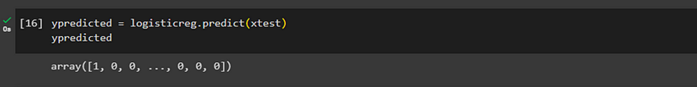
Now we predict values, to our x-Test data. “ypredicted” is the set of predicted data by our model using predict(x).

5.Accuracy

Now we must check the accuracy of our model using accuracy_score. For that, we are using our predicted dataset and the actual data set corresponding to the x-Test dataset.

Or we can look at the confusion matrix of our model. Our model works well if we get the Confusion matrix to be TruePositive and/or TrueNegative.

Here we get a 2-D confusion matrix. Because there are 2 classes in our output, which are, ‘1’, and ‘0’.

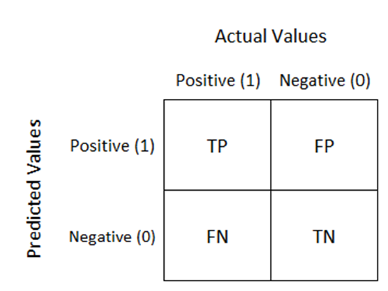
The confusion matrix consists of four basic characteristics (numbers) that are used to define the measurement metrics of the classifier in machine learning These four numbers are:

1. TP (True Positive): TP represents the number of patients who have been properly classified to have malignant nodes, meaning they have the disease.
2. TN (True Negative): TN represents the number of correctly classified patients who are healthy.
3. FP (False Positive): FP represents the number of misclassified patients with the disease but actually they are healthy. FP is also known as a Type I error.
4. FN (False Negative): FN represents the number of patients misclassified as healthy but actually they are suffering from the disease. FN is also known as a Type II error.

Performance metrics of an algorithm are accuracy, precision, recall, and F1 score, which are calculated on the basis of the above-stated TP, TN, FP, and FN.

The accuracy of an algorithm is represented as the ratio of correctly classified patients (TP+TN) to the total number of patients (TP+TN+FP+FN).

The precision of an algorithm is represented as the ratio of correctly classified patients with the disease (TP) to the total patients predicted to have the disease (TP+FP).

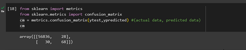
confusion matrix

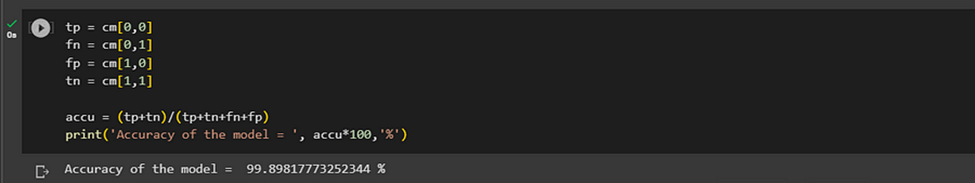
assigning values from the matrix to separate variables and then finding accuracy

Now, we have predicted a model with an accuracy of 99.89% to predict if a transaction is fraudulent or not. Complete code: Fraud_Detection.ipynb

[back to topic list]

Naive Bayes

When we have a data point and want to discover which group it belongs to, Naive Bayes can help. A data point’s likelihood of falling into a particular category is determined by this.

The foundation for Naive Bayes is a mathematical principle known as Bayes’ theorem, which enables us to revise our beliefs or predictions in light of fresh information. Calculating the likelihood that a data point falls into each category involves combining the data point’s evidence with our prior knowledge of the categories.

Now, you might be wondering why it’s called “Naive.” Well, Naive Bayes makes a simplifying assumption called the “naive” assumption. It assumes that the different features or characteristics of the data point are independent of each other, meaning that they don’t influence each other.

This assumption allows the calculation to be performed more easily and efficiently in machine learning

Based on the estimated probabilities, we can use Naive Bayes to predict the category of a data point. By examining the connections and patterns within the characteristics of the data point, it aids in the classification and categorization of data.

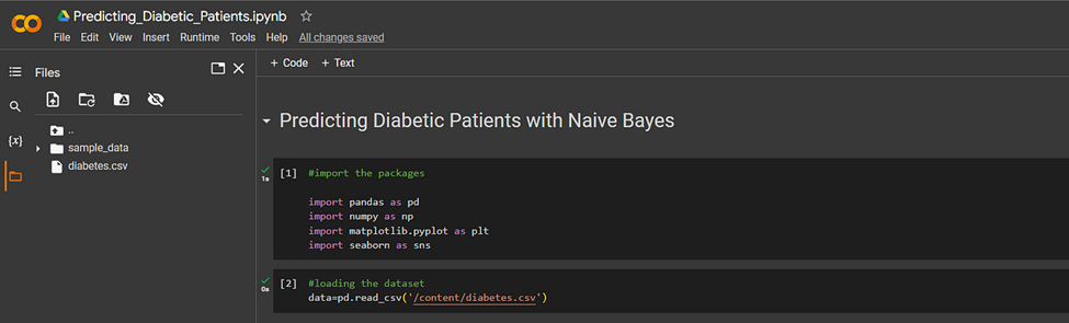
Let us start training a model with an example data set, diabetes.csv.

In this demonstration, we will train a model to detect if the patient is diabetic or not. Now we have an idea about how to work on Google Colab and add necessary .csv files and read them.

1.Understanding the data

We upload our data file to Colab and read the file.

Then we take a look at the data that we just loaded with (pandas.DataFrame.head), (pandas.DataFrame.tail), (pandas.DataFrame.shape), etc.

2.Detect and treat any possible missing values

Then we must see if there are any missing values in the data set.

data.isna()
data.isna().any()
data.info()
data.describe()

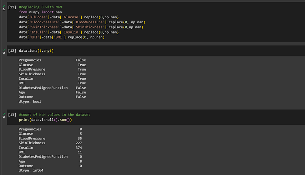
We can see, although there are no missing values, there are unusual 0.00 values in columns ‘Glucose’, ‘BloodPressure’, ‘SkinThickness’, ‘Insulin’. This must be wrong. Because in any case, Glucose level or blood pressure in the human body cannot be 0. So we must replace these wrong values.

Missing values or wrong values are common in dealing with real-world problems when the data is aggregated over a long time stretch from disparate sources and reliable machine learning modeling demands careful handling of missing data. One strategy is imputing the missing values, with mean, median or mode.

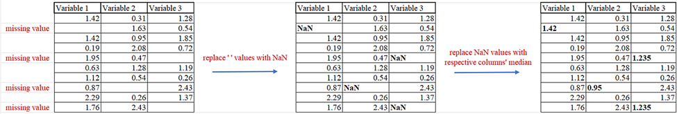
First, we replace the 0.0 value with NaN values. 

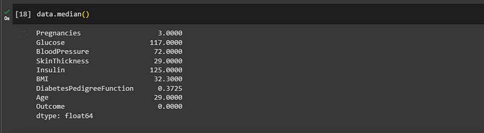
Then we get the median values of each column, ‘Glucose’, ‘BloodPressure’, ‘SkinThickness’, ‘Insulin’. And impute those values in the place of NaN values.

So, our new medians of the columns look like this. We can see they have not changed at all.

3.Outlier detection and treatment

An outlier is a data point that is unusually high or low compared to the other nearby data points. It stands out because it doesn’t follow the general pattern of the rest of the data in a dataset or graph.

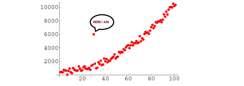
Outlier of a data set
https://medium.com/analytics-vidhya/its-all-about-outliers-cbe172aa1309

Identifying and dealing with outliers is a crucial task in data preprocessing. Outliers can have a detrimental impact on statistical analysis and the training of machine learning algorithms, leading to lower accuracy. Therefore, it is essential to detect and handle outliers effectively.

Boxplots are a great way of detecting outliers. Once the outliers have been detected, they can be imputed with the 5th and 95th percentiles.

#using boxplots to find outliers
plt.figure(figsize=(20,15))

plt.subplot (4,4,1)
plt.title('Pregnancies')
sns.boxplot (data['Pregnancies'])

plt.subplot (4,4,2)
plt.title('Glucose')
sns.boxplot (data['Glucose'])

plt.subplot (4,4,3)
plt.title('BloodPressure')
sns.boxplot (data['BloodPressure'])

plt.subplot (4,4,4)
plt.title('SkinThickness')
sns.boxplot (data[ 'SkinThickness'])

plt.subplot (4,4,5)
plt.title('Insulin')
sns.boxplot (data['Insulin'])

plt.subplot (4,4,6)
plt.title('BMI')
sns.boxplot (data['BMI'])

plt.subplot (4,4,7)
plt.title('DiabetesPedigreeFunction')
sns.boxplot(data['DiabetesPedigreeFunction'])

plt.subplot (4,4,8)
plt.title('Age')
sns.boxplot(data['Age'])

Box plots

The little dots we can see in these box plots are the ouliers of the data set.

Percentile capping is an approach used to handle outlier values by replacing them with specific percentiles. Observations below a lower limit are replaced with the 5th percentile value, while observations above an upper limit are replaced with the 95th percentile value from the same dataset.

This technique helps to mitigate the impact of outliers on data analysis.

data['Pregnancies']=data['Pregnancies'].clip(lower=data['Pregnancies'].quantile(0.05), upper=data['Pregnancies'].quantile(0.95))
data['Glucose']=data['Glucose'].clip(lower=data['Glucose'].quantile(0.05), upper=data['Glucose'].quantile(0.95))
data['BloodPressure']=data['BloodPressure'].clip(lower=data['BloodPressure'].quantile(0.05), upper=data['BloodPressure'].quantile(0.95))
data['SkinThickness']=data['SkinThickness'].clip(lower=data['SkinThickness'].quantile(0.05), upper=data['SkinThickness'].quantile(0.95))
data['Insulin']=data['Insulin'].clip(lower=data['Insulin'].quantile(0.2), upper=data['Insulin'].quantile(0.85))
data['BMI']=data['BMI'].clip(lower=data['BMI'].quantile(0.05), upper=data['BMI'].quantile(0.95))
data['DiabetesPedigreeFunction']=data['DiabetesPedigreeFunction'].clip(lower=data['DiabetesPedigreeFunction'].quantile(0.05), upper=data['DiabetesPedigreeFunction'].quantile(0.95))
data['Age']=data['Age'].clip(lower=data['Age'].quantile(0.05), upper=data['Age'].quantile(0.95))

Now the box plots show the dataset with lesser outliers.

4.Model training 

We use train_test_split to separate out training data and test data. Here, the dependent variable, y, is ‘Outcome’ which is patient is diabetic or not. And independent variable, x, is all the other columns without the ‘Outcome’ column.

from sklearn.model_selection import train_test_split

x=data.drop(['Outcome'],axis=1)
y=data['Outcome']

xtrain,xtest,ytrain,ytest=train_test_split(x,y,test_size=0.2,random_state=40)

x and y variables

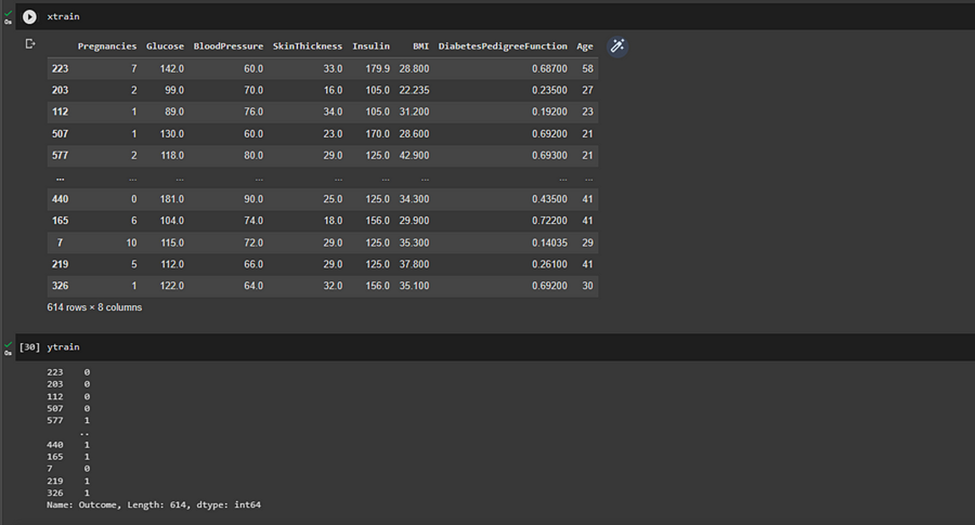
x-Train and y-Train data sets

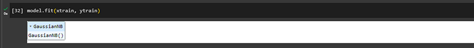
Now we create a Gaussian Classifier model using sklearn.naive_bayes

from sklearn.naive_bayes import GaussianNB
#CREATE GUASSIAN CLASSIFIER
model = GaussianNB()

And fit our x-Train and y-Train data to this model and train it.

 5.Predicting

Now we predict a set of data corresponding to the x-Test data set.

6. Accuracy test

So our model has an accuracy of 76.62%.

Complete code: Predicting_Diabetic_Patients.ipynb

[back to topic list]

Decision Tree

Decision trees are fantastic tools for solving classification problems in machine learning, as they possess the ability to precisely organize and order different classes. Think of a decision tree as a flow chart that guides us through a series of decisions to classify data points accurately. The tree structure starts with a “trunk” and branches out into “branches” and further extends into “leaves.”

As we traverse this tree, the data points are systematically divided into increasingly similar categories. The “trunk” represents the initial set of all data points, and as we move towards the “branches,” the data points become more refined and separated based on their features. Finally, at the “leaves,” we arrive at finely defined categories where the data points share significant similarities.

This hierarchical structure of decision trees allows for the creation of categories within categories, providing an organic and granular approach to classification. The beauty of decision trees lies in their ability to achieve this level of classification with limited human intervention. The tree learns and discerns patterns in the data on its own, guided by the given features and their relationships.

By leveraging decision trees, we can classify and categorize data points effectively, making informed decisions based on their unique characteristics. This algorithm empowers us to extract valuable insights and predictions from complex datasets, promoting better understanding and decision-making.

Let us start training a model with an example data set, iris.csv.

In this demonstration, we will train a model to detect the species of the Iris flower in Jupyter Notebook.

1. Reading and understanding the data

First, we import pandas and read the .csv file using pd.read_csv().

And visualize the data using matplotlib pyplot

from matplotlib import pyplot as plt

plt.figure(figsize=(15,10))

plt.subplot(4,4,1)                         #subplot 1
plt.hist(iris['SepalLengthCm'],color='g')  #plotting a histogram
plt.title('Distribution of sepal length')  #setting title
plt.xlabel('Sepal length')                 #setting xlabel

plt.subplot(4,4,2)
plt.hist(iris['PetalLengthCm'],color='g')
plt.title('Distribution of petal length')
plt.xlabel('Petal length')

plt.subplot(4,4,3)
plt.hist(iris['SepalWidthCm'],color='g')
plt.title('Distribution of sepal width')
plt.xlabel('Sepal width')

plt.subplot(4,4,4)
plt.hist(iris['PetalWidthCm'],color='g')
plt.title('Distribution of petal width')
plt.xlabel('Petal width')

plt.show()

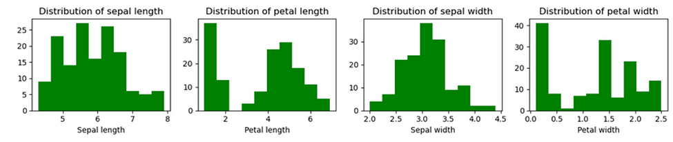
Histograms representing each independent variable in the data set

2.Detect and treat any possible missing values

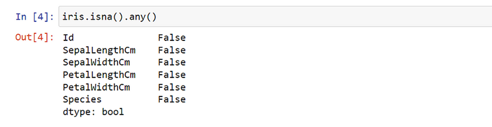
In this dataset, we do not have any missing values. But if we do, we need to treat them as we did previously.

from numpy import nan

iris.replace('', np.nan) #if you have empty data

#replacing with median
iris.fillna(iris.median(),inplace=True) 

#or delete the rows and columns with NULL values
iris = iris.dropna(axis=0) #drop row
iris = iris.dropna(axis=1) #drop column

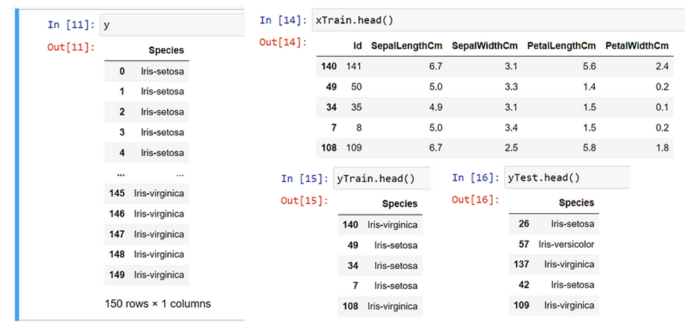
3. Model training data preparation

##setting our dependant and independant variables

y=iris[['Species']]
x=iris.drop(['Species'],axis=1)

##setting our test and training data
from sklearn.model_selection import train_test_split
xTrain,xTest,yTrain,yTest = train_test_split(x,y,test_size=0.3)

4. Model training

Here we use DecisionTreeClassifier() from sklearn.tree

from sklearn.tree import DecisionTreeClassifier
dtc = DecisionTreeClassifier()

#training the model with our data
dtc.fit(xTrain,yTrain)

5.Predicting

Let us predict data with our x-Test data. We get an array for ‘predicted’.

predicted = dtc.predict(xTest)
predicted

6.Accuracy

To calculate the accuracy of the model we take the confusion matrix of the predicted data and our y-Test data set.

from sklearn.metrics import confusion_matrix

confusion_matrix(yTest,predicted)

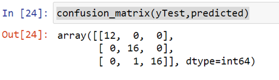
Here we get a 3-D confusion matrix. Because there are 3 classes in our output, which are, ‘Iris-setosa’, ‘Iris-versicolor’, and ‘Iris-virginica’. 

How to know the TP, TN, FP, and FN values as in the above case?

In the multi-class classification problem, we won’t get TP, TN, FP, and FN values directly as in the binary classification problem. For validation, we need to calculate for each class.

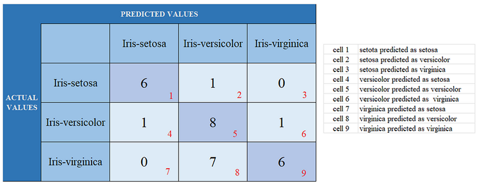
Setosa: TP = cell 1, FN = ( cell 2 + cell3 ), FP = ( cell 4 + cell 7 ), TN = (cell 5 + cell 6 + cell 8 + cell 9)
Versicolor: TP = cell 5, FN = (cell 4 +cell 6), FP = (cell 2 + cell 8), TN = (cell 1 + cell 3 + cell 7 + cell 9)
Virginica: TP = cell 9, FN = ( cell 7 + cell 8), FP = (cell 3 + cell 6), TN = (cell 1 + cell 2 + cell 4 + cell 5)

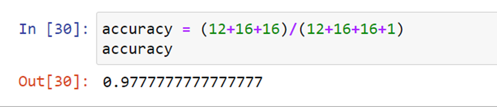
The accuracy of the model would be the addition of TPs in all sectors.

accuracy = (S: TP + Ve: TP + Vi: TP) / (addition of all cell values )

Complete Code: Decision_Tree_Demo

we learned most of concepts in machine learning.

In the next article, we will do demonstrations on Regression models in Machine Learning.

Thank you and Happy Reading! 

[back to topic list]

 Follow For More.

References

https://monkeylearn.com/blog/classification-algorithms/

https://u-next.com/blogs/machine-learning/popular-regression-algorithms-ml/