

Imagine ! with your eyes closed, a world in which computers are able to see and understand their surroundings in the same ways that people do. Sounds fun, no? That’s what we’re going to look into together.

Have you ever thought about that how your mobile phone recognizes your face? or have you ever thought about how Facebook suggest when we tag others when we upload a photo?.how does the robot understand the environment?
Computer vision comes to play.
Before diving into computer vision, we need to know the basics about images. then we can move into coding. we use Python language and the OpenCV library. we will cover the most of topics about computer vision in this article
Topic list (click to jump )
- image formats
- colours
- resolution
- spyder and miniconda
- Reading images
- imread flags
- processing images 1.0
- imwrite()
- Changing colourspace
- Finding colours
- Real-time colour detection
image formats
first, let’s look at what the image is. In computer vision, we deal with digital photos. Then what is the digital photo?JPEG, PNG, GIF, TIFF and RAW are the basic image formats. If you consider a video, it is actually a series of pictures. we going to process videos also.
colours
We work with ones and zeros because the world is digital. it means that binary integers are used to collect data. Additionally, the primary colours used in the digital world are red, green, and blue. By combining these primary colours, we can get secondary and other colours.
in this article, we mainly talk about two colour models.
RGB colour model
To better comprehend the RGB colour scheme, let’s open Paint.

We can make new colours by increasing the values for the RED, BLUE, and GREEN sections. Generally, we can set each section’s maximum value to 255 (decimal).and the minimum value is 0 (decimal). because we use an 8-bit colour scheme. that means we use 8 bits for the RED value and another 8 bit for BLUE and another 8 bit for green.
| coor | RED value(8 bit) | GREEN value(8 bit) | colour(8 bit) |
| Red | 255 | 0 | 0 |
| Green | 0 | 255 | 0 |
| Blue | 0 | 0 | 255 |
| White | 255 | 255 | 255 |
| Black | 0 | 0 | 0 |
| Orange | 255 | 165 | 0 |
| Purple | 128 | 0 | 128 |
HSV colour model
The H stands for Hue, S stand for saturation and V stands for value.

Hue is used to describing the color itself, like red, blue, or green. Think of a colour wheel with all the hues arranged in a circle on it. Where colour is on this wheel is indicated by its hue. Consider a rainbow as an illustration; each colour indicates a different hue.
Saturation is a term used to describe a colour’s intensity or purity. Consider it to be the intensity or vibrancy of a hue. Fully saturated colours appear rich and pure. However, as the saturation falls, the colour begins to appear more washed out or faded.
Value describes a colour’s brightness or darkness. It controls how a colour appears to our eyes—how light or dark. If we consider shades of gray, for instance, the value defines whether it is light gray or a dark gray. The value in the HSV colour model runs from black to white, and changing it affects the colour’s overall brightness.
In the next parts, we’ll talk more about this HSV model.
The resolution
now let’s talk about resolution.

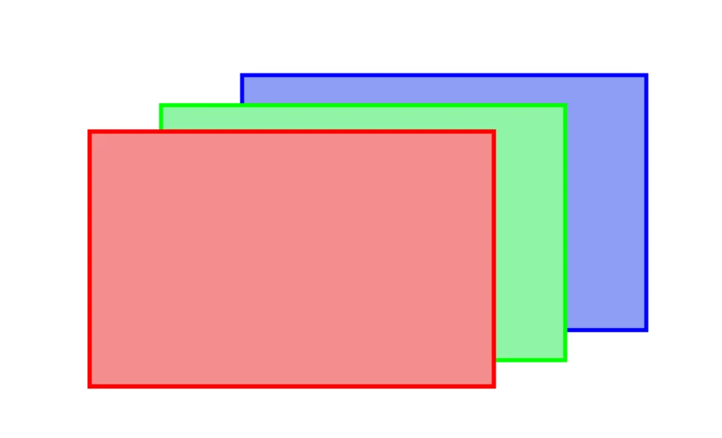
Think about Square Rule Notebook. You can see little squares if you zoom in on your photograph. and colours are added to those squares. in computer vision, we name each pixel by a combination of columns and rows.
[ column, raw ].

Spyder and Miniconda
We use Spyder ide and Miniconda to run our Python programs.
you have to run these commands in your Anaconda terminal
conda create --name spyder5_1env --clone base
conda activate spyder5_1envconda install spyder-kernels=2.3conda install numpy
pip install opencv-python
then you have to enter the Python interpreter

Reading Images
Let’s write our first Python code in computer vision. First, you can create your own image using software like Paint or any other graphics editing software of your choice. then name as test1.jpg.(it is better to use low resolution image )
import cv2 # Import the OpenCV library for computer vision tasks
import matplotlib.pyplot as plt # Import the matplotlib library for plotting images
import numpy as np # Import the numpy library for numerical operations
BGR_im = cv2.imread("test1.jpg")
# Read the image file "test1.jpg" and store it in BGR_im
# Here, BGR_im represents the image in the BGR (Blue-Green-Red) color format
cv2.namedWindow("BGR image", cv2.WINDOW_NORMAL)
# Create a named window to display the BGR image
# cv2.WINDOW_NORMAL allows resizing of the window if necessary
cv2.imshow("BGR image", BGR_im)
# Display the BGR image in the created window
# The image will be displayed using the OpenCV library's imshow() function
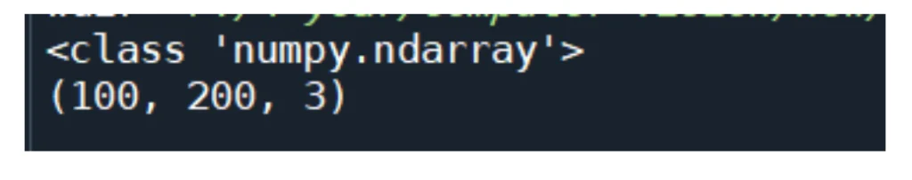
print(type(BGR_im))
print(BGR_im.shape)
cv2.waitKey(0) & 0xFF
# Wait for a key press to continue the execution
# The waitKey() function waits indefinitely for a key event to occur.
# The returned value is bitwise ANDed with 0xFF to ensure compatibility across different platforms
cv2.destroyAllWindows()
# Close and destroy all the previously created windows
# This ensures that all the windows created by imshow() are closed properly and memory is released
Note: it is better to use low-resolution images for testing our first computer vision practical. (like 200 * 100 jpg). you know that the image is a combination of arrays.
We define the variable as BGR_im because when we use the OpenCV library to display an image, it reads the image in the reverse order of the colour layers, namely Blue-Green-Red (BGR) instead of the more commonly used Red-Green-Blue (RGB) format. Therefore, to accurately represent the image and avoid colour distortions, we store it in the BGR_im variable.
this is what your output looks like.

A 3-dimensional numpy array brings up the variable “BGR_im”. It represents a three-layer or three-channel image. There are 100 rows and 200 columns in each channel. The blue colour channel is represented by the first layer, the green colour channel by the second layer, and the red colour channel by the third layer.
Furthermore, we can utilize the ‘matplotlib.pyplot’ library to display our image. when using this library, the image is read in the proper Red-Green-Blue (RGB) order. This means that the colour channels are interpreted in the correct sequence. not like opencv.
let’s move into the next practical in our computer vision journey.
cv2.imread(filename[,flags])
we can read images under three different conditions.
| Integer flag | flag | description |
| 1 | cv2.IMREAD_COLOR | Loads a color image. Default |
| 0 | cv2.IMREAD_GRAYSCALE | Loads image in grayscale mode |
| -1 | cv2.IMREAD_UNCHANGED | Loads a colour image. Default |
In certain computer vision scenarios, we encounter situations where we need to read an image in a different manner.
Processing images practical 1.0
let’s split the RGB layers and then print it as our second computer vision practical.
import cv2  # Import the OpenCV library
import matplotlib.pyplot as plt  # Import the matplotlib library
import numpy as np  # Import the numpy library

bgr_im = cv2.imread("test1.jpg")  # Read the image file "test1.jpg" and store it in the variable bgr_im
# The image is read in BGR (Blue-Green-Red) format by default

[B, G, R] = cv2.split(bgr_im)  # Split the BGR image into its individual color channels

# Create named windows to display the images
cv2.namedWindow("BGR image", cv2.WINDOW_NORMAL)
cv2.namedWindow("B_channel", cv2.WINDOW_NORMAL)
cv2.namedWindow("G_channel", cv2.WINDOW_NORMAL)
cv2.namedWindow("R_channel", cv2.WINDOW_NORMAL)

# Display the images in their respective windows
cv2.imshow("BGR image", bgr_im)
cv2.imshow("B_channel", B)
cv2.imshow("G_channel", G)
cv2.imshow("R_channel", R)

cv2.waitKey(0) & 0xFF  # Wait for a key press to continue the execution

# The waitKey() function waits indefinitely for a key event to occur.
# The returned value is bitwise ANDed with 0xFF to ensure compatibility across different platforms

cv2.destroyALLWindows()

# Close and destroy all the previously created windows
# This ensures that all the windows created by imshow() are closed properly and memory is released
this is what your output looks like

And you may observe the continued presence of borders within the image, which can be attributed to the image format utilized. In the upcoming sections on computer vision, we will delve into the techniques of utilizing code to eliminate borders from images.
Now we consider about data type and shape of the B, G, and R variables.
print(type(B))
print(B.shape)
print(type(G))
print(G.shape)
print(type(R))
print(R.shape)
Then our final output will be like this
<class 'numpy.ndarray'>
(100, 200)
<class 'numpy.ndarray'>
(100, 200)
<class 'numpy.ndarray'>
(100, 200)
That indicates that these variables possess two dimensions. And we previously discussed black = 0,0,0 and while = 255,255,255, in three-dimensional cases. in this, we only have one value.
then the white space area should definitely be set to 255. Therefore, if we take into consideration the B array, the blue rectangle’s area should also be 255. This G and R array is identical to others.
These layers appear grayscale because each layer represents the brightness or intensity values of the respective colour channel. Grayscale images use shades of grey, ranging from black (lowest intensity) to white (highest intensity), to show the intensity values. When printed independently, the R, G, and B layers are shades of grey since they primarily contain intensity information rather than colour information.
that is why we notice that these layers appear grey!
let’s explore some basic OpenCV functions
imwrite
you can save the final output using imwrite()
import cv2
import matplotlib.pyplot as plt
import numpy as np

BGR_im = cv2.imread("test1.jpg", 1)  # Read image in color mode
b, g, r = cv2.split(BGR_im)  # Split BGR image
im2 = cv2.merge([r, g, b])  # Merge channels (convert to RGB)

cv2.namedWindow("BGR image", cv2.WINDOW_NORMAL)  # Create resizable window
cv2.imshow("BGR image", BGR_im)  # Show BGR image

cv2.imwrite("test2.png", im2)  # Save modified image as PNG

cv2.waitKey(0) & 0xFF  # Wait for key press to exit
cv2.destroyAllWindows()  # Close all windows
Changing colourspace
Changing an image’s colour space is sometimes necessary for computer vision. Two colour spaces (RGB and HSV) were covered in the previous section. Let’s now look at techniques for converting between several colour spaces.
There are several common techniques for converting an RGB image to a grayscale image, including the average method and the weighted method.
average method
Grayscale = (1/3) R+(1/3) G+(1/3) B
In this method, we sum up the values of R (red), G (green), and B (blue) in their respective layers, and then divide the sum by 3. This averaging process ensures an equal contribution from each colour channel to obtain the final result.
import cv2
import matplotlib.pyplot as plt
import numpy as np

BGR_im = cv2.imread("van.jpg",1) #READING IMAGE
b,g,r = cv2.split(BGR_im)


cv2.namedWindow("BGR image",cv2.WINDOW_NORMAL)
cv2.imshow("BGR image",BGR_im)

gray_im = np.uint8((1 / 3 )* r + (1 / 3 )* g + (1 / 3) * b)  # Convert to grayscale

cv2.namedWindow("gray image",cv2.WINDOW_NORMAL)
cv2.imshow("gray image",gray_im)


cv2.waitKey(0) &0xFF
cv2.destroyAllWindows()
This is your final output look like

The Weighted Method
The average method is simple but it doesn’t function as expected since our eyes process RGB colors differently. Green light is the most sensitive to us. red light and blue light less than green light. This calls for the distribution of the colours to have different weights. then takes use weighted technique.
Grayscale = 0.299R + 0.587G + 0.114B
This equation is a commonly used standard in various computer vision applications.
import cv2
import matplotlib.pyplot as plt
import numpy as np

BGR_im = cv2.imread("cat.jpg",1) #READING IMAGE
b,g,r = cv2.split(BGR_im)


cv2.namedWindow("BGR image",cv2.WINDOW_NORMAL)
cv2.imshow("BGR image",BGR_im)

gray_im1 = np.uint8((1 / 3 )* r + (1 / 3 )* g + (1 / 3) * b)  # Convert to grayscale

cv2.namedWindow("gray image 1",cv2.WINDOW_NORMAL)
cv2.imshow("gray image 1",gray_im1)

gray_im2 = np.uint8(0.299*r + 0.587*g + 0.114*b)  # Convert to grayscale

cv2.namedWindow("gray image 2",cv2.WINDOW_NORMAL)
cv2.imshow("gray image 2",gray_im2 )


cv2.waitKey(0) &0xFF
cv2.destroyAllWindows()
this is what your output looks like
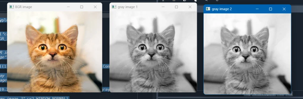
you can see there are some small changes in “gray image 2”
cv2.cvtColor
this a simple function to convert RGB images to gray
import cv2
import matplotlib.pyplot as plt
import numpy as np

BGR_im = cv2.imread("woman.jpg",1) #READING IMAGE
b,g,r = cv2.split(BGR_im)


cv2.namedWindow("BGR image",cv2.WINDOW_NORMAL)
cv2.imshow("BGR image",BGR_im)

gray_im1 = np.uint8((1 / 3 )* r + (1 / 3 )* g + (1 / 3) * b)  # Convert to grayscale


cv2.namedWindow("gray image 1",cv2.WINDOW_NORMAL)
cv2.imshow("gray image 1",gray_im1)

gray_im2 = np.uint8(0.299*r + 0.587*g + 0.114*b)  # Convert to grayscale

cv2.namedWindow("gray image 2",cv2.WINDOW_NORMAL)
cv2.imshow("gray image 2",gray_im2 )

gray_im3 = cv2.cvtColor(BGR_im,cv2.COLOR_BGR2GRAY)  # Convert to grayscale

cv2.namedWindow("gray image 3",cv2.WINDOW_NORMAL)
cv2.imshow("gray image 3",gray_im3  )


cv2.waitKey(0) &0xFF
cv2.destroyAllWindows()
this is what your output looks like

you can see there are some small changes in “gray image 3”
Finding colours in the image
in this section, we move into a few advanced concepts in computer vision. we are going to find colours using our computer vision.
To work with the HSV colour space in coding, we need to understand the techniques and methods specific to handling HSV colour space.
In this colour space, we need to provide three values, similar to the RGB colour space, but with different ranges. The ranges for Value and Saturation are from 0 to 1, while the range for Hue is from 0 to 359.
but In our programmes, HSV colour space, the hue range is typically [0, 179], the saturation range is [0, 255], and the value range is [0, 255].
It’s important to note that different software may utilize different scales for these ranges. Therefore, when comparing OpenCV values with values from other software, it may be necessary to normalize or adjust these ranges accordingly.
import cv2
import matplotlib.pyplot as plt
import numpy as np

BGR_im = cv2.imread("sky2.jpg", 1)  # Read BGR image
HSV_im = cv2.cvtColor(BGR_im, cv2.COLOR_BGR2HSV)  # Convert image to HSV color space

Blue_ub = np.array([130, 255, 255])  # Upper threshold for blue color in HSV
Blue_ln = np.array([110, 50, 50])  # Lower threshold for blue color in HSV

mask = cv2.inRange(HSV_im, Blue_ln, Blue_ub)  # Create a mask for blue color pixels

# Create named windows for visualization
cv2.namedWindow("BGR_im", cv2.WINDOW_NORMAL)
cv2.namedWindow("mask", cv2.WINDOW_NORMAL)
cv2.namedWindow("mask_im", cv2.WINDOW_NORMAL)

cv2.imshow("BGR_im", BGR_im)  # Display the original BGR image
cv2.imshow("mask", mask)  # Display the binary mask

cv2.waitKey(0) & 0xFF  # Wait for a key press to exit
cv2.destroyAllWindows()  # Close all windows
we focus on the blue colour and our output looks like this.

Actually, this basic concept can be further developed in more advanced ways within the field of computer vision. There are numerous techniques and algorithms available that can enhance the accuracy, efficiency, and robustness of image processing and analysis tasks.
Here is a helpful dictionary representing HSV color space values for computer vision coding
color_dict_HSV = {
    'black': [[180, 255, 30], [0, 0, 0]],
    'white': [[180, 18, 255], [0, 0, 231]],
    'red1': [[180, 255, 255], [159, 50, 70]],
    'red2': [[9, 255, 255], [0, 50, 70]],
    'green': [[89, 255, 255], [36, 50, 70]],
    'blue': [[128, 255, 255], [90, 50, 70]],
    'yellow': [[35, 255, 255], [25, 50, 70]],
    'purple': [[158, 255, 255], [129, 50, 70]],
    'orange': [[24, 255, 255], [10, 50, 70]],
    'gray': [[180, 18, 230], [0, 0, 40]]
}
you can edit previous code using this dictionary
import cv2
import matplotlib.pyplot as plt
import numpy as np

color_dict_HSV = {
    'blue': [[130, 255, 255], [110, 50, 50]],
    'green': [[89, 255, 255], [36, 50, 70]],
    'red1': [[180, 255, 255], [159, 50, 70]],
    'red2': [[9, 255, 255], [0, 50, 70]],
    'yellow': [[35, 255, 255], [25, 50, 70]],
    'purple': [[158, 255, 255], [129, 50, 70]],
    'orange': [[24, 255, 255], [10, 50, 70]],
    'black': [[180, 255, 30], [0, 0, 0]],
    'white': [[180, 18, 255], [0, 0, 231]],
    'gray': [[180, 18, 230], [0, 0, 40]]
}

BGR_im = cv2.imread("sky2.jpg", 1)  # Read BGR image
HSV_im = cv2.cvtColor(BGR_im, cv2.COLOR_BGR2HSV)  # Convert image to HSV color space

color_name = 'blue'  # Select the desired color from the dictionary
color_range = color_dict_HSV[color_name]  # Get the HSV range for the selected color

color_ub = np.array(color_range[0])  # Upper threshold for selected color in HSV
color_lb = np.array(color_range[1])  # Lower threshold for selected color in HSV

mask = cv2.inRange(HSV_im, color_lb, color_ub)  # Create a mask for the selected color

# Create named windows for visualization
cv2.namedWindow("BGR_im", cv2.WINDOW_NORMAL)
cv2.namedWindow("mask", cv2.WINDOW_NORMAL)
cv2.namedWindow("mask_im", cv2.WINDOW_NORMAL)

cv2.imshow("BGR_im", BGR_im)  # Display the original BGR image
cv2.imshow("mask", mask)  # Display the binary mask

cv2.waitKey(0) & 0xFF  # Wait for a key press to exit
cv2.destroyAllWindows()  # Close all windows
Real-time colour detection
This is another simple computer vision exercise where you can detect colours in real-time using your webcam.
import cv2

# Create a VideoCapture object to access the webcam
cap = cv2.VideoCapture(0)

while True:
    # Read frames from the webcam
    ret, frame = cap.read()

    if not ret:
        break

    # Convert the frame to the HSV color space
    hsv_frame = cv2.cvtColor(frame, cv2.COLOR_BGR2HSV)

    # Define the color ranges for detection
    lower_blue = (100, 50, 50)
    upper_blue = (130, 255, 255)

    # Create a mask for the specified color range
    mask = cv2.inRange(hsv_frame, lower_blue, upper_blue)

    # Apply the mask to the frame
    result = cv2.bitwise_and(frame, frame, mask=mask)

    # Display the original frame and the resulting masked frame
    cv2.imshow('Original', frame)
    cv2.imshow('Masked', result)

    # Break the loop if 'q' is pressed
    if cv2.waitKey(1) & 0xFF == ord('q'):
        break

# Release the VideoCapture object and close the windows
cap.release()
cv2.destroyAllWindows()
This is what your final output looks like.

This article provides an introduction to computer vision for beginners. Through straightforward code examples, we’ll go over fundamental ideas including colour spaces, resolutions, and colour recognition. Although there are other Python libraries for computer vision. but in this article, we focused on OpenCV. You will ultimately be able to recognize colours in a video stream. We’ll cover advanced computer vision facts and methods in upcoming articles.